Calculating adjusted OHLC values

This article describes a general procedure to calculate adjusted OHLC values for a time series, and provides its implementation.

I was motivated to investigate this after reading Giulio Botazzi's Download historical data using Alpha Vantage, which offers great insight into this matter.

Software

Sample implementation written in Python; required packages:

• requests
• matplotlib
• pandas

I also recommend using a Jupyter notebook to try out the code.

Stock price data

Free data provided by Alpha Vantage.

Adjustment methodology

We'll be using the standard Boston CRSP method. The idea is to calculate an adjustent factor to account for both splits and dividend hand-outs. We can then use these multipliers to calculate adjusted OHLC values; for instance:

adjusted close = close * split factor * dividend factor

These adjustment factors compound over time, so we should calculate them iteratively going back in time:

adjustment factor_today = f_tomorrow * adjustment factor_tomorrow
f_i = split or dividends factor for day i

Implementation

Start by importing the necessary libraries.

import requests
import csv
import pandas as pd
          

Get price data

Add your Alpha Vantage API key here.

API_KEY = 'my-alpha-vantage-api-key'
          

Download full historical daily price data for IBM.

symbol = 'IBM'
url = 'https://www.alphavantage.co/query?' \
    'function=TIME_SERIES_DAILY_ADJUSTED&datatype=csv&outputsize=full&' \
    f'symbol={symbol}&apikey={API_KEY}'
response = requests.get(url)                           # issue request
response_text = response.content.decode('utf-8')       # get response text
csv_reader = csv.reader(response_text.splitlines())    # init csv reader
time_series = [ row for row in csv_reader ][1:]        # skip column names row
          

The resulting time_series is just an array where each item holds price data for one day. This daily data is also an array with the following fields:

0. timestamp
1. open
2. high
3. low
4. close
5. adjusted_close
6. volume
7. dividend_amount
8. split_coefficient

split_coefficient

The new-number-of-shares to old-number-of-shares ratio. This value is different than one only on split dates; i.e. on days the price and shares were adjusted for the split.

dividend_amount

The per-share value of dividends paid. Stocks start trading without their dividends on the ex-dividend date, so only on these days will the dividend_amount be different than zero.

Calculate adjustment factors

In this next part, we'll be adding 2 more columns to our time_series:

9. split_factor
10. dividend_factor

Note that Alpha Vantage's data is in reverse chronological order.

# for the most recent day, split_factor = dividend_factor = 1
split_factor = 1
dividend_factor = 1

# append split_factor and dividend_factor columns to most recent day
time_series[0].append(split_factor)
time_series[0].append(dividend_factor)

# calculate for the rest of the time series 
for i in range(1, len(time_series)):

    today = time_series[i]                     # current day
    tomorrow = time_series[i - 1]              # day chronologically after

    dividend_amount = float(tomorrow[7])       # dividends and split coefficient
    split_coefficient = float(tomorrow[8])     # AlphaVantage columns 7 and 8, 0-based index

    # recalculate split factor for current day
    split_factor /= split_coefficient

    # recalculate dividends factor
    close = float(today[4])
    dividend_factor *= (close - dividend_amount) / close

    # add split_factor and dividend_factor columns 
    today.append(split_factor)
    today.append(dividend_factor)
          

Calculate OHLC adjusted values

Let's calculate the adjusted close as an example, and add it as another column in our time_series:

11. my_adjusted_close

for i in range(0, len(time_series)):
    today = time_series[i]
    close = float(today[4])        # current day's close
    split_factor = today[9]        # split and dividend factors in new columns 9 and 10
    dividend_factor = today[10]
    
    # factor in split and dividends for adjusted close value
    # should be equal to AlphaVantage's adjusted_close in column 5
    my_adjusted_close = close * split_factor * dividend_factor
    today.append(my_adjusted_close)
          

Plot the time_series

Let's get the data in the proper chronological order.

time_series.reverse()
          

Then, prepare a pandas dataframe.

columns = [ 'timestamp', 'open', 'high', 'low', 'close', 'adjusted_close', 
            'volume', 'dividend_amount', 'split_coefficient', 
            'split_factor', 'dividend_factor', 'my_adjusted_close' ]

df = pd.DataFrame(time_series, columns = columns)           # create data frame
df = df.set_index('timestamp')                              # set timestamp as index
df['close'] = df['close'].astype(float)                     # cast close and adjusted_close
df['adjusted_close'] = df['adjusted_close'].astype(float)   # need type float to plot
          

We can now plot close, adjusted_close (Alpha Vantage), and my_adjusted_close.

df[['close', 'adjusted_close', 'my_adjusted_close']].plot(figsize = (16, 8));
          

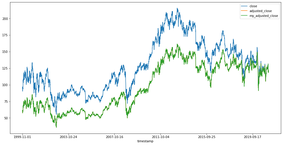
Alpha Vantage's adjusted_close and my_adjusted_close are overlapping. Let's get a close-up of the first 16 data points and compare the values.

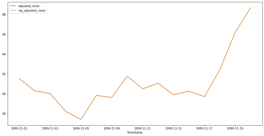
Alpha Vantage states they are also using the CRSP approach in their support page, so that checks out.

Alternative calculation method?

If we try the above procedure to calculate adjusted close values for Microsoft (MSFT), we get the following result:

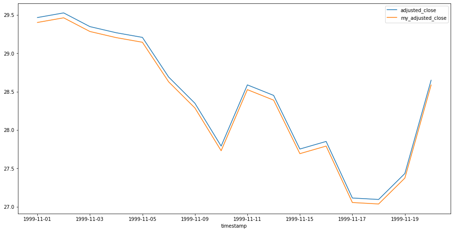
I was tempted to disregard the difference as just a rounding error. However, if we were to calculate the dividend_factor using the next day's open value instead of the previous close...

    # recalculate dividends factor
    open_price = float(tomorrow[1])
    dividend_factor *= open_price / (dividend_amount + open_price)
          

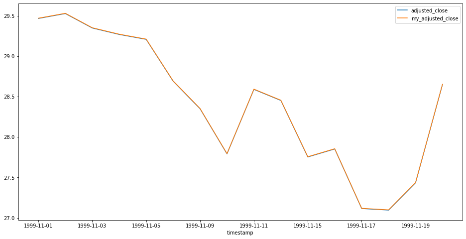
It looks like Alpha Vantage is using another formula in this case. Go figure.

Appendix: Adjusted shares and volume

We need to use the inverse adjustment factor for the number of shares and volume.

for i in range(0, len(time_series)):
    today = time_series[i]
    volume = float(today[6])       # current day's volume
    split_factor = today[9]
    dividend_factor = today[10]
    
    # apply inverse adjustment factor for volume
    my_adjusted_volume = volume / (split_factor * dividend_factor)
    today.append(my_adjusted_volume)
          

Conclusion

For consistency, calculate your own adjusted OHLC values for technical analysis.